
Gradient Descents
Gradient Descents
In this post, we are going to discuss Gradient Descents; what it is and how to use it. Gradient Descent is used in many machine learning algorithms to find the local minimum in differentiable functions where there is a linear relationship. It goes hand in hand with optimization problems. In this tutorial, we will focus on linear regressions. A linear regression is used to model the relationship between one or more variables. In our case, we have an input $x$ and an output $y$, but we do not know the slope $m$ or the intercept $b$.
\[y = mx + b\]To build our model, we need to tune two parameters, namely $m$ and $b$ . To do so, we need to use the mean squared error (MSE) as our loss function. This function measures the average squared difference between the estimated values and the actual value. We expect this to be 0 if our predicted values equal our actual value.
\[MSE =\frac{1}{N}\Sigma_{i=1}^{n}(Y_{i}-\hat Y_{i})^{2}\]Therefore, we will need optimize the MSE for a linear regression using the gradient descent. A gradient is defined as follows:
\[\nabla J(\theta) = [\frac{\partial J}{\partial\theta_{1}},\frac{\partial J}{\partial\theta_{2}},...,\frac{\partial J}{\partial\theta_{p}}]\]The gradient descent is defined in the following equation. The algorithm will iterate over and over using the gradient descent to find new values of $m$ and $b$ . This will continue until MSE converges to zero, letting us know that our predicted values equal to our actual values.
\[\theta_{n + 1} =\theta_{n} -\eta\nabla J(\theta_{n})\]Let’s first solve for $\nabla J(\theta_{n})$ by plugging in the MSE equation and finding the partial derivatives with respect to $m$ and $b$.
\[MSE =\frac{1}{N}\Sigma_{i=1}^{n}(y_{i}-(mx_{i}+b))^{2}\] \[f(m,b) =\frac{1}{N}\Sigma_{i=1}^{n}(y_{i}-(mx_{i}+b))^{2}\] \[\frac{\partial f(m,b)}{\partial m} =\frac{1}{N}\Sigma_{i=1}^{n}-2(y_{i}-(mx_{i}+b))\frac{\partial f}{\partial m}(mx_{i}+b))\] \[\frac{\partial f(m,b)}{\partial m} =\frac{1}{N}\Sigma_{i=1}^{n}-2x_{i}(y_{i}-(mx_{i}+b))\] \[\frac{\partial f(m,b)}{\partial b} =\frac{1}{N}\Sigma_{i=1}^{n}-2(y_{i}-(mx_{i}+b))\frac{\partial f}{\partial b}(mx_{i}+b))\] \[\frac{\partial f(m,b)}{\partial b} =\frac{1}{N}\Sigma_{i=1}^{n}-2(y_{i}-(mx_{i}+b))\]Now we have our two final equations. We can begin implementing them.
\[\hat m = m -\eta(\frac{1}{N}\Sigma_{i=1}^{n}-2x_{i}(y_{i}-(mx_{i}+b)))\] \[\hat b = b -\eta(\frac{1}{N}\Sigma_{i=1}^{n}-2(y_{i}-(mx_{i}+b)))\]We will input two vectors $x$ and $y$ and solve for $m$ and $b$. In addition, we set a learning rate, $\eta$ of 0.001. This controls the magnitude of the gradient. If it is too large, we will miss the minima, but if it is too small, the number of iterations will increase. For this function, we will iterate 10,000 times and break the loop if $MSE\le\epsilon$, $\epsilon = 0.001$.
gradient_descent <- function(x,y, epsilon = 0.001, lr = 0.001, steps = 10000){
  epsilon = 0.0001
  m = runif(1) #Initialize a random number
  b = runif(1) #Initialize a random number
  N = length(x)
  log = c()
  mseloss = c()
  for (step in 1:steps){
    f = y - (m*x + b) #Subtracting the estimated value from the actual value
    mseloss = c(mseloss, sum(f ** 2) / N)
    dm <- -2 / N * sum(x %*% f)
    db <- -2 / N * sum(f)
    m = m - lr * dm
    b = b - lr * db
    log = rbind(log, c(m,b))
    if (sum(f ** 2) / N <= epsilon){ #stop the algorithm once we have converged to zero
      break
    }
  }
  list = list('m' = m, 'b' = b, 'steps' = step, 'log' = log, 'mseloss' = mseloss)
  return(list).
We can initialize a simple example by setting x = c(1,2,3,4,5) and
y = 2 * x. We expect m = 2 and b = 0.
x = c(1,2,3,4,5)
y = 2 * x
ptm <- proc.time()
res <- gradient_descent(x,y)
proc.time() - ptm
##    user  system elapsed
##   0.723   0.454   1.185
res$m
## [1] 1.992251
res$b
## [1] 0.02797554
cat('The predicted values are:', head(res$m * x + res$b))
## The predicted values are: 2.020227 4.012478 6.004729 7.99698 9.989232
cat('\nThe actual values are:', head(y))
##
## The actual values are: 2 4 6 8 10
We can observe convergence by plotting the MSE against the number of iterations.
library(ggplot2)
df <- data.frame('iters' = 1:res$steps, 'mseloss' = res$mseloss)
ggplot(df, aes(x = iters, y = mseloss)) + geom_point() + theme_minimal() + ylab('MSE Loss')
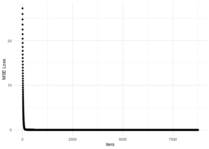
It appears to converge early but continues on to meet our requirement of $MSE\le\epsilon$ . Let’s repeat this with a larger data set. We would expect this to take longer.
x = runif(10000)
y = 2 * x
ptm <- proc.time()
res <- gradient_descent(x,y)
proc.time() - ptm
##    user  system elapsed
##   2.542   1.425   4.022
res$m
## [1] 1.577939
res$b
## [1] 0.2254082
cat('The predicted values are:', head(res$m * x + res$b))
## The predicted values are: 0.8785615 0.6359393 1.200908 0.628451 1.231726 0.5944415
cat('\nThe actual values are:', head(y))
##
## The actual values are: 0.8278561 0.5203383 1.236423 0.5108471 1.275484 0.4677408
df <- data.frame('iters' = 1:res$steps, 'mseloss' = res$mseloss)
ggplot(df, aes(x = iters, y = mseloss)) + geom_point() + theme_minimal() + ylab('MSE Loss')
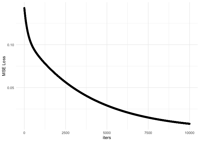
As you can see, the predicted values don’t match the actual values. In addition, the MSE loss does not converge. This suggests we may need more iterations. Let’s try with 50,000 iterations.
ptm <- proc.time()
res <- gradient_descent(x,y, steps = 50000)
proc.time() - ptm
##    user  system elapsed
##   9.538   5.721  15.327
res$m
## [1] 1.965497
res$b
## [1] 0.01842688
cat('The predicted values are:', head(res$m * x + res$b))
## The predicted values are: 0.8320013 0.5297885 1.23352 0.5204611 1.271906 0.4780985
cat('\nThe actual values are:', head(y))
##
## The actual values are: 0.8278561 0.5203383 1.236423 0.5108471 1.275484 0.4677408
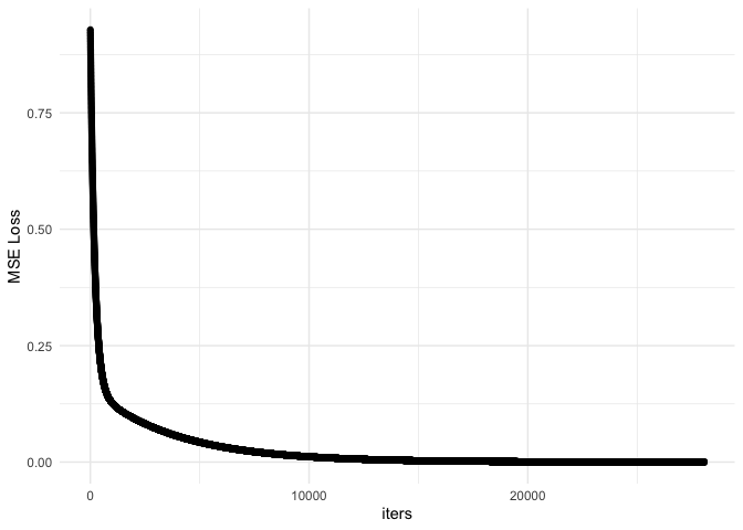
df <- data.frame('iters' = 1:res$steps, 'mseloss' = res$mseloss)
ggplot(df, aes(x = iters, y = mseloss)) + geom_point() + theme_minimal() + ylab('MSE Loss')
Comparing to Stochastic Gradient Descent
Now it looks like we have converged and reached an optimal value. However, the time it took was much longer. To wrap up, we were able to determine a suitable $m$ and $b$ to satisfy our optimization problem. However, this algorithm can be slow if we are working with large matrices. In that case, we can use Stochastic Gradient Descent and use only a subset of the matrix with one sample at a time for the optimization.
Let’s see what this would look like.
s_gradient_descent <- function(x,y, epsilon = 0.001, lr = 0.001, steps = 10000, batch_size = 1){
  epsilon = 0.0001
  m = runif(1) #Initialize a random number
  b = runif(1) #Initialize a random number
  log = c()
  mseloss = c()
  for (step in 1:steps){
    index <- sample.int(length(y), batch_size)
    N = length(index)
    Xs <- x[index]
    Ys <- y[index]
    f = Ys - (m*Xs + b) #Subtracting the estimated value from the actual value
    mseloss = c(mseloss, sum(f ** 2) / N)
    dm <- -2 / N * sum(Xs %*% f)
    db <- -2 / N * sum(f)
    m = m - lr * dm
    b = b - lr * db
    log = rbind(log, c(m,b))
    if (sum(f ** 2) / N <= epsilon){ #stop the algorithm once we have converged to zero
      break
    }
  }
  list = list('m' = m, 'b' = b, 'steps' = step, 'log' = log, 'mseloss' = mseloss)
  return(list).
With the above function, we will only be using a subset of our data for optimization. In this case, I will set it to 100. Feel free to play around with the parameters.
ptm <- proc.time()
sgd_res <- s_gradient_descent(x,y, steps = 50000, batch = 100)
proc.time() - ptm
##    user  system elapsed
##   4.532   2.952   7.543
sgd_res$m
## [1] 1.961864
sgd_res$b
## [1] 0.02037149
cat('The predicted values are:', head(sgd_res$m * x + sgd_res$b))
## The predicted values are: 0.8324419 0.5307878 1.233218 0.5214777 1.271534 0.4791934
cat('\nThe actual values are:', head(y))
##
## The actual values are: 0.8278561 0.5203383 1.236423 0.5108471 1.275484 0.4677408
As you can see, we nearly cut out run time in half by just using stochastic gradient descent.