Introduction to R and RStudio

What is R?

R is a language and environment for statistical computing and graphics. It is widely used for a variety of statistical analysis (i.e., linear and nonlinear modeling, classical statistical tests, clustering, etc.). We can also use R for data visualization and producing figures for presentations. R is freely available and has a large collection of developed packages of different tools. Overall, R is a powerful tool that can be used to handle big data, perform statistics, and visualize results, while enabling end-users to easily develop tools and packages for customized functionality.

What is RStudio?

While R, also called “base R”, itself is an interpreted computer language and comes with a terminal, ease of use and more functionality is introduced when using RStudio, an open source Integrated Development Environment (IDE). Rather than using a terminal, RStudio provides a graphical user interface that is platform agnostic and integrates additional packages, project management, version control, and notebooks.

Getting started with R and RStudio

The Comprehensive R Archive Network or CRAN actively maintains and develops R. It also hosts a repository of R packages that enhances the base functionality of R. To get started, base R can be installed on either Linux, macOS, or Windows by going to the CRAN homepage.

To use R, you need to open a terminal window and type R and press enter. You will see some text denoting the R version and some helpful functions. To quit, type q() and press enter.

Rather than work in a terminal, RStudio is the way to use R like how many use Microsoft Word to prepare documents. Download RStudio for free here and follow the installation instructions. Once installed, proceed to opening RStudio, typically done by clicking on the RStudio icon.

Once you open RStudio, you will see four main panes. Each will contain different information. You can see my screen below.

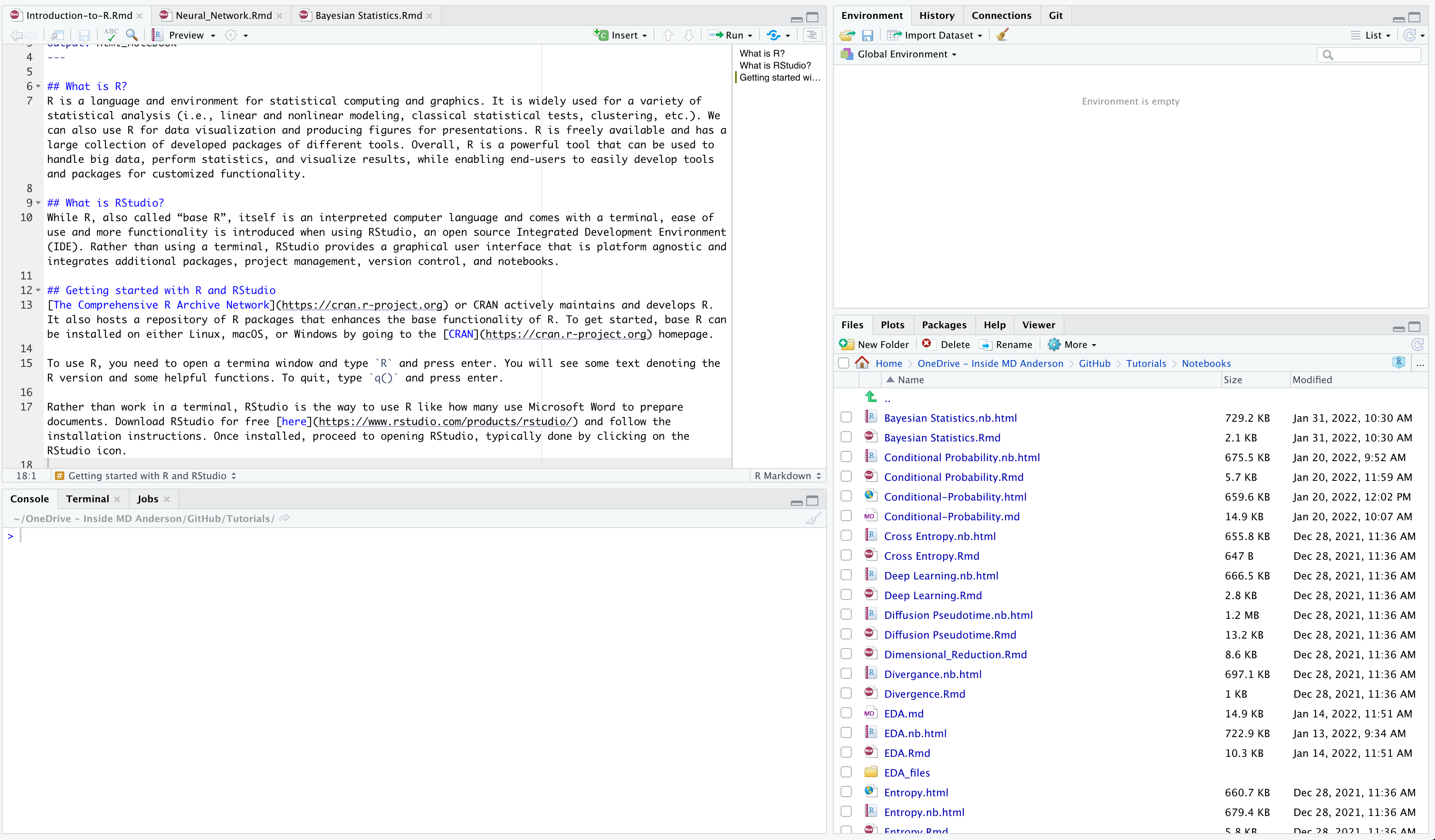
Starting from the top left pane and going from left to right, we have the descriptions of each pane below:

1. Source Editor: This pane is where you can write R scripts or notebooks. You can write in other programming languages if you wanted to as well. Each document will have its own tab. Code written here can be run with the Run command.
2. Environment: This pane displays objects, variables, and functions that are generated in your R session. There is also a history of all code that was run.
3. Console: This pane is where you can type commands and interactively run R code. The output will display in the console.
4. Files, Plots, Packages, Help, Viewer: This pane has several tabs that are important.
   • Files: This tab shows the structure and content of a directory on your computer. This could be your working directory or a directory that you manually navigated to.
   • Plots: This tab will display plots or figures as an output from the console.
   • Packages: This tab contains a list of all packages that are installed. Packages that are loaded in your R session will have a checked box.
   • Help: This tab reveals the help pages for an R package or function.
   • Viewer: This tab shows compiled R Markdown documents.

Starting a new project in RStudio

When working with R, it is always a good idea to create a new project directory. This will help you keep your files and data organized by project.

To get started: 1. Open RStudio 2. Go to the File menu and select New Project. 3. In the New Project window, choose New Directory. Then, choose New Project. Name your new directory. You can use a name like, Intro-to-R, and then “Create the project as subdirectory of:” in a location of your choice. 4. Click on Create Project. 5. The project should open up automatically in Rstudio.

We can view our working directory by using the function getwd()

getwd()

## [1] "/Users/dtruong4/Desktop/Intro-to-R"

Your working directory will be the location where R will automatically look for files. If you want to find files in a different location, you will either need to provide the full path or type the path in relation to the working directory. Files that you output will automatically save into your working directory unless a path is provided.

To organize your working directory, it is highly recommended to generate sub-folders like data/ or results/. You can do so in the Files tab and select New Folder.

Basic math calculations in R

Below are some of the most common math calculations that can be done in R.

Operation	Symbol
Addition	a + b
Subtraction	a - b
Multiplication	a * b
Division	a / b
Exponent	a ^ b
Remainder	a %% b
Integer Division	a %/% b

For instance, here is an example of addition.

5 + 3

## [1] 8

Functions in R

R has several pre-built functions. For instance, we can use sum() instead of the + symbol for addition.

sum(1,3) #This gives the sum of 1 and 3

## [1] 4

We can also call the R documentation for a function by using ? before the function name. The documentation will show up under the Help tab. It contains information regarding description, usage, and arguments for a function.

?sum #Find the R Documentation for sum()

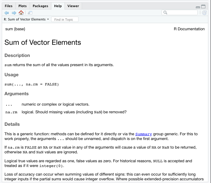
We can see that sum() can return the sum of more than two values.

sum(1,2,3,4,5)

## [1] 15

Math functions in R

In addition to the basic calculations, there are many common pre-built math functions in R.

Operation	Function
Square root	sqrt()
Logarithm	log()
Logarithm, base 10	log10()
Exponential	exp()
Summation	sum()
Round	round()
Mean	mean()
Median	median()
Minimum	min()
Maximum	max()

#What is the square root of 4?
sqrt(4)

## [1] 2

#Can we round 3.14?
round(3.14)

## [1] 3

Defining variables

A key aspect of programming is defining variables. We store data or values as variables so that we can use in other functions or recall it at a later time. It allows us to save time by storing the data and not having to re-calculate it again. R has two assignment operators for defining variables: <- and =. The operator <- can be used anywhere, whereas the operator = is only allowed at the top level.

x <- 1

#What is in `x`?
x

## [1] 1

y = 15.3

#What is in `y`?
y

## [1] 15.3

#What is in x + y?
x + y 

## [1] 16.3

We can also define variables within functions.

sqrt(y <- 5)

## [1] 2.236068

#What is in `y`?
y

## [1] 5

However, we cannot use the = to do so. This is because functions already have pre-defined arguments that the function is looking for. In this case, sqrt() is looking for the argument x, not y.

sqrt(y = 5) 

## Error in sqrt(y = 5): supplied argument name 'y' does not match 'x'

Instead, we can do the following:

sqrt(x = y <- 5) #Here we define y as 5 and pass y into x 

## [1] 2.236068

sqrt(x = 5) #Here we pass 5 into x

## [1] 2.236068

Importantly, when defining variable names, ensure that you use an informative name. This enables yourself and others when reviewing code to know how the variable was used. For instance, we used x and y in the examples, but their meaning is unknown. Something like country_population or room_capacity provides better definition for a variable.

R Data Types

There are different types of data in R, which can be stored as a variable. Below is a table of some of the most commonly used data types.

Data Type	Definition	Example
numeric	Any number value	3.14
integer	Any whole number value	42
character	Any number of ASCII characters	"Hello world!"
	defined within quotation marks
logical	A value of TRUE or FALSE	TRUE
factor	A categorical type of data	#> [1] Male Male Male Female Female
		#> Levels: Male Female

The function class() can be used to find out the type of data that you are dealing with.

x <- 3
class(x)

## [1] "numeric"

x <- TRUE
class(x)

## [1] "logical"

Vectors

Vectors are a data structure in R containing one or more values. In fact, you may have noticed a [1] in the output of x. This indicates that it is a vector of length 1.

length(x) #This function gives you the length of a vector

## [1] 1

We use the function c() to define a vector with multiple elements. The c stands for combine.

my_first_vector <- c(1,2,3,4,5) #We can also do this with the following, 1:5 instead of c()
my_first_vector

## [1] 1 2 3 4 5

We can add more elements to the same vector.

my_first_vector <- c(my_first_vector, 6,7)
my_first_vector

## [1] 1 2 3 4 5 6 7

We can call specific elements in a vector by using a process called indexing. Basically, we can subset specific elements of a vector for further analysis. We do this by defining which position we want in brackets [] after the vector.

#Let's take out the 3rd element
my_first_vector[3]

## [1] 3

What if we wanted to select multiple elements? We can use another vector with the positions we want.

#Let's take out the 2nd and 4th elements
my_first_vector[c(2,4)]

## [1] 2 4

We can also do the opposite and select all elements but a single or multiple element by using -.

#Let's keep all but the 5th element
my_first_vector[-5]

## [1] 1 2 3 4 6 7

#Let's keep all but the 1st and 3rd elements
my_first_vector[-c(1,3)]

## [1] 2 4 5 6 7

Importantly, R functions are typically vectorized. This means that the function will perform its operation on all elements of the vector without having to loop through for each element.

my_first_vector

## [1] 1 2 3 4 5 6 7

my_first_vector * 2

## [1]  2  4  6  8 10 12 14

We can also test some of math functions we listed above.

mean(my_first_vector) #This gives the mean of a numeric vector

## [1] 4

min(my_first_vector) #This gives the minimum numeric value in a vector

## [1] 1

max(my_first_vector) #This gives the maximmum numeric value in a vector

## [1] 7

Relational and Logical Operators

In R, there are relational operators that compare values between two variables. Typically, these are numerical equalities or inequalities. The result of comparison is a Boolean value.

Operator	Description
<	less than
<=	less than or equal to
>	greater than
>=	greater than or equal to
==	equal to
!=	not equal to
%in%	is ‘in’ a given vector

#Is 3 greater than 5?
3 > 5

## [1] FALSE

We can use the %in% operator to determine if a given value is in a vector.

#Is 5 in 1 through 10?
5 %in% 1:10

## [1] TRUE

#Is 'a' in c('a','b','c')?
'a' %in% c('a','b','c')

## [1] TRUE

There are also logical operators which connect two or more expressions depending on the meaning of the operator. These are typically combined with relational operators.

Operator	Description
|	OR
&	AND
!	NOT

#Is 3 greater than 1 and 5?
3 > 1 & 3 > 5

## [1] FALSE

#Is 3 greater than 1 or 5?
3 > 1 | 3 > 5

## [1] TRUE

User-Written Functions

We can build custom functions to perform operations that are not pre-built in base R. Custom functions can include pre-built or other custom functions. In fact, many pre-built functions are functions of other pre-built functions.

my_function <- function(arg1, arg2,...){
  statements
  return(object)
}

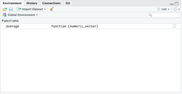
Let’s make a function that finds the average of a numeric vector.

average <- function(numeric_vector){
  out <- sum(numeric_vector)/length(numeric_vector)
  return(out)
}

Once we have created our function, you will see it under the Functions section in the Environment tab.

Let’s test our function below.

average(c(1,2,3))

## [1] 2

What happens if we put a non-numeric vector?

average(c('a', 'b', 'c'))

## Error in sum(numeric_vector): invalid 'type' (character) of argument

While R has an error message for some cases, we can also build your own error function with a custom message.

average <- function(numeric_vector){
  if (class(numeric_vector) != 'numeric') #condition to throw the error
    out <- 'This is not a numeric vector' #The custom error message
  else
    out <- sum(numeric_vector)/length(numeric_vector) 
  return(out)
}

average(c('a', 'b', 'c'))

## [1] "This is not a numeric vector"

We can also view the code of any function by typing it without the (). This can help you understand how a function works, especially if it created by someone else.

average

## function(numeric_vector){
##   if (class(numeric_vector) != 'numeric') #condition to throw the error
##     out <- 'This is not a numeric vector' #The custom error message
##   else
##     out <- sum(numeric_vector)/length(numeric_vector) 
##   return(out)
## }

Best Practices

1. Document your code, thoughts, and decision making. Keep this in a .Rmd or .r file. Use # for commenting. This will aid in reproducible of your code for yourself and others.
2. Create and work inside an R project. This helps with code and data organization.
3. Use informative naming for variables. Try to stay from x, y, or similar.
4. Do create functions to simplify your code.
5. Practice and keep learning!

Additional Resources

• Introduction to R and Rstudio: Harvard Bioinformatics
• Introduction to R and RStudio: Alex Lemonade Stand
• Introduction to R and RStudio: Yale CRC